Soil Type Prediction

To demonstrate the capabilities and advantages of machine learning to my peers, I worked on an underutilized algorithm, binary classification, on a soil dataset. Without using the scikit-learn machine learning library, I developed a logistic regression code with the following objective in mind:

To demonstrate how blowcounts can be used to predict soil type, with enough data.

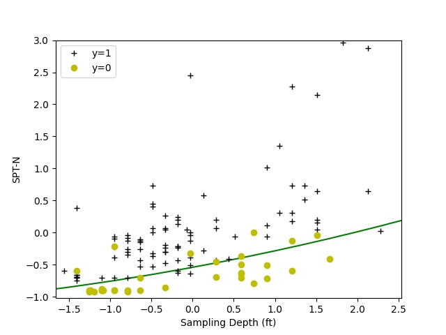
The training dataset was prepared using several data reduction and transformation techniques, such as feature selection, polynomial feature mapping, and normalization. By using a higher-order, non-linear model, the algorithm achieves training accuracy of about 90% with up to five training features: Depth, N-value, N_6”, N_12”, and N_18”. A decision boundary for Depth and N-value are presented below to illustrate the class separation.

89.68% accuracy with two features

91.27% accuracy with three features

90.48% accuracy with five features

This exercise is inspired by Andrew Ng’s ML Speciliazation on Coursera. If you are interested in more details, please continue to read and visit the repository:
[GitHub/soil-type-predictions]

Data Limitations

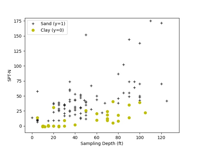
The dataset consists of nine sets of SPT data collected at a site within the San Francisco Bay Area. Groundwater was as shallow as 5 feet below ground surface (bgs) at this site. The thickness of the artificial fill was in the range of 5 to 9 feet bgs, overlying marsh and alluvial deposits. These soil borings were drilled with the mud-rotary method to maximum depth of about 130 feet, and the soil samples were logged by an experienced geologist or engineer. No bedrock was encountered in these borings. For the simplicity of this project, soils are categorized as either sand or clay. Plotting the SPT N-value against the depth at which soil samples were collected, we see that clayey soils tend to have lower blowcounts compared to sandy soils with increasing depths. This is reasonable given that natural clays submerged at shallow depth are very soft to soft, except one with an N-value of 14 at a depth of 5 feet bgs, which can be fill or clay crust. At greater depths, blowcounts in clayey soil are still comparatively lower than sandy soil. Hint: the shallower and deeper geological clay deposits shown here are Young Bay Mud and Old Bay Clay, respectively.

Data Transformation

The logistic regression algorithm makes use of regularization and gradient descent to minimize the cost. Therefore, an inherent issue is numerical stability or convergence. In order to better quantify the data, several extra steps are needed to prepare the training set prior to model training.

In very soft soil, a commonly encountered sampling condition is the weight of hammer (WoH). WoH represents the lowering of the sampling device to the sampling depth at which the combined weight of the drilling rod(s) and soil sampler penetrate the whole 18 inches without driving the hammer. Therefore, no blowcount is noted. To distinguish the difference between WoH and zero (0-0-0) blowcounts, WoH is set as a “-1” N-value in the dataset.

To further prepare training data for logistic regression, two other techniques were implemented: (i) normalization and (ii) feature mapping. Data normalization using z-score has been applied to transform features to a similar scale to improve the performance and training stability of the model. In this context, “features” refer to variables of interest such as “depth” and “N-value”. Feature mapping is slightly more complicated and harder to explain. In brief, feature mapping refers to the transformation of training data from a lower-dimensional to a higher-dimensional space, where it can be more effectively analyzed or classified. In other words, it nonlinearizes or converts data to higher order like X², X³ etc. One of the more tedious tasks is cracking the feature mapping algorithm for multiple features, such as the PolynomialFeatures( ) in sklearn. Turns out that the PolynomialFeatures( ) simply loops through the specified “degree” with combinations function such as itertools.combinations_with_replacement( ):

import math
import itertools

X = [2,3,4]
degree = 3
res = []

for i in range(1, degree+1):
	C = list(itertools.combinations_with_replacement(X, i)) 
	
	for j in range(len(C)):       
		res.append(math.prod(C[j]))

print(res)
print(len(res))

# [2, 3, 4, 4, 6, 8, 9, 12, 16, 8, 12, 16, 18, 24, 32, 27, 36, 48, 64]
# 19

# degree = 1, 3 elems: [2, 3, 4]
# degree = 2, 6 elems: [4, 6, 8, 9, 12, 16]
# degree = 3, 10 elems: [8, 12, 16, 18, 24, 32, 27, 36, 48, 64]

Thumbnail photo credit: Makc76
Last update: 10/2023